
Nerve cell firing in vivo
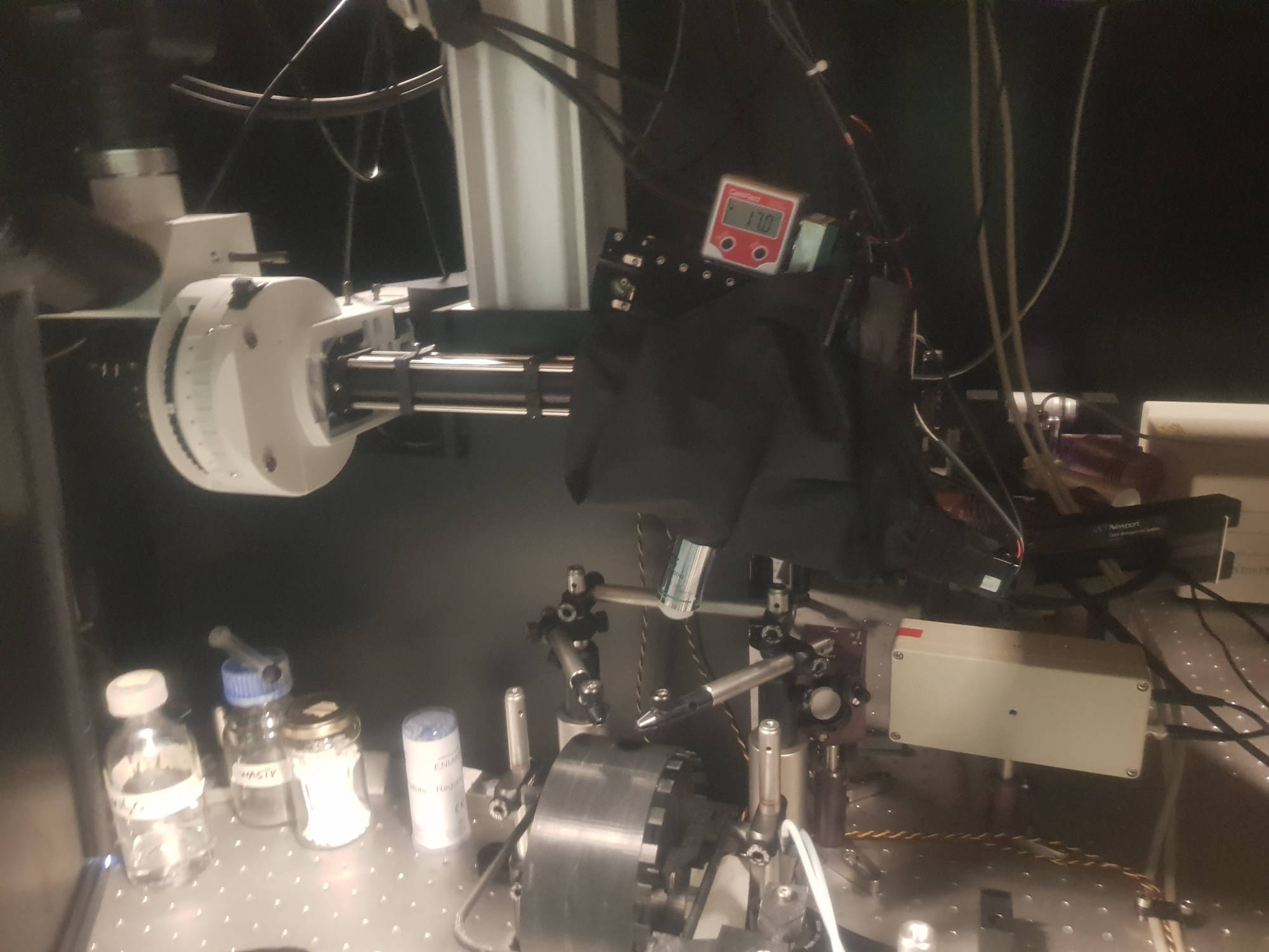
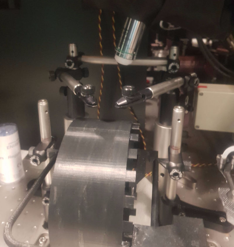
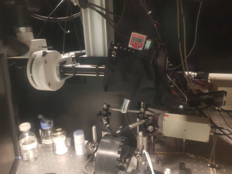
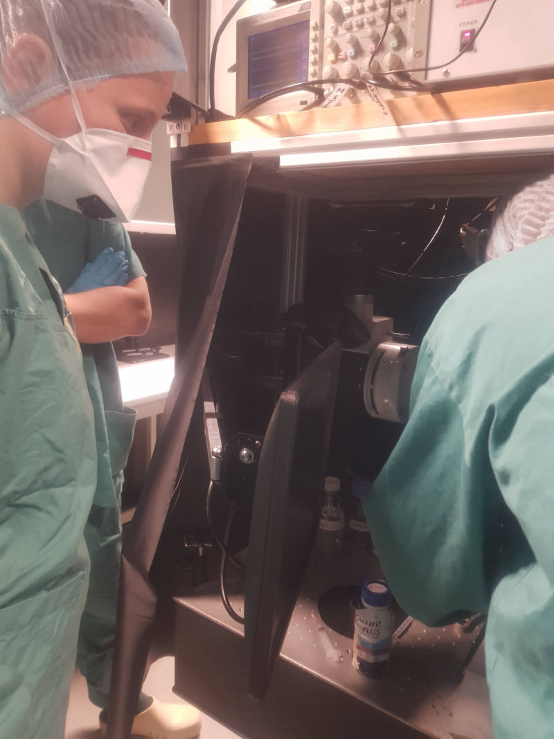
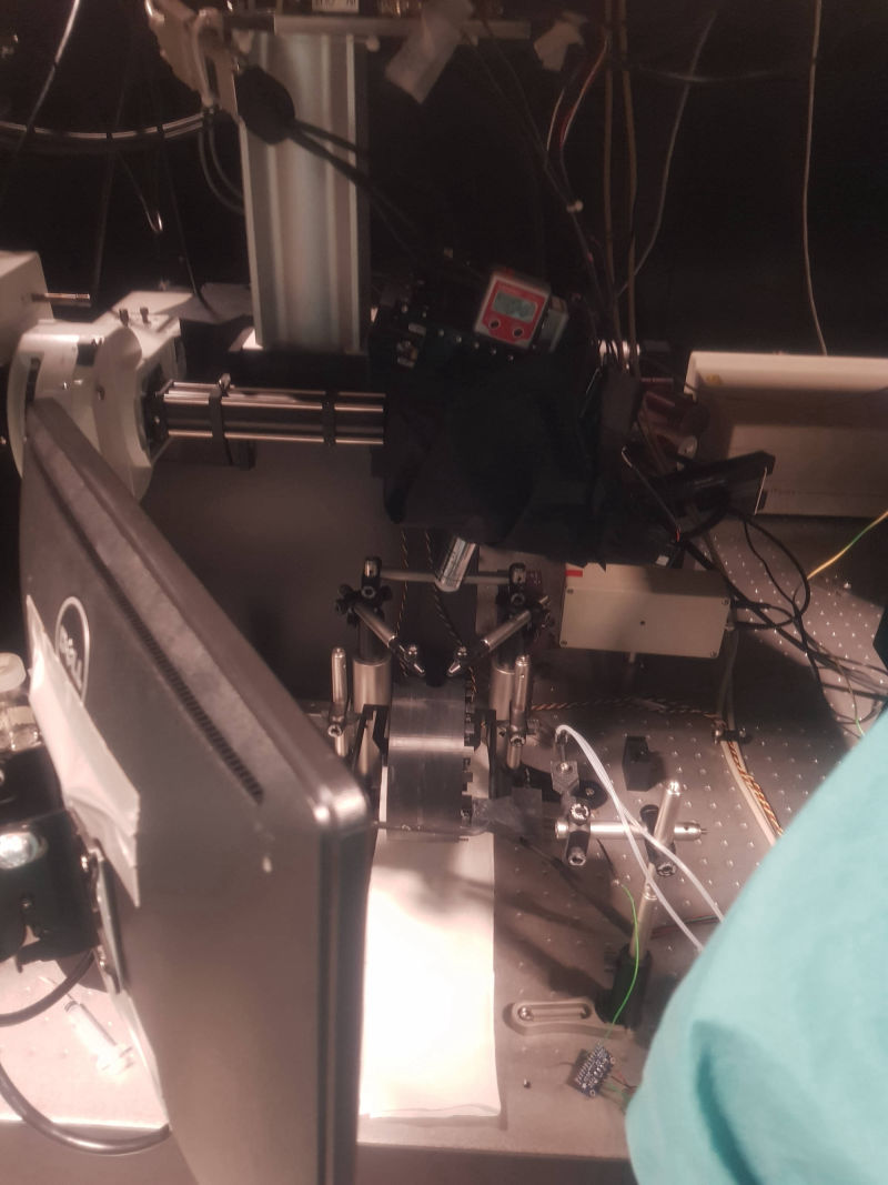
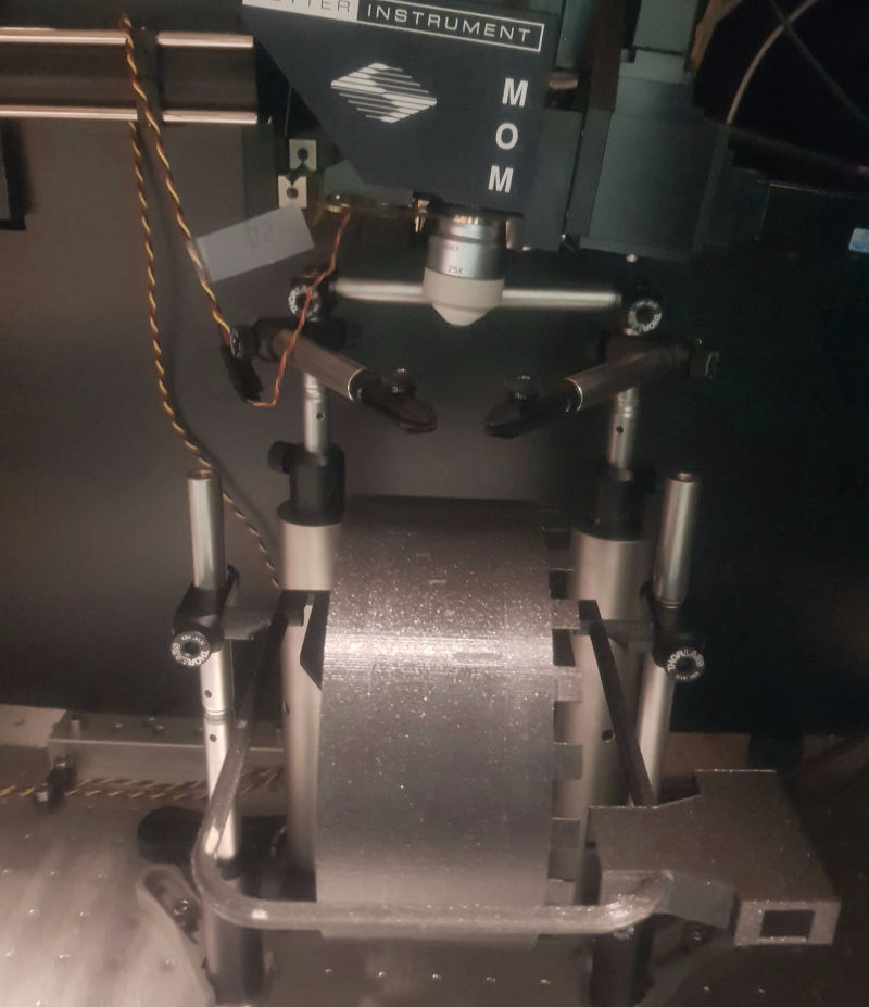
We were allowed to follow a fantastic experiment where two-photon fluorescence microscopy was used to image calcium dynamics during nerve cell firing in the visual cortex of a mouse running on a treadmill!!
Reviews about the two-photon technique in neuroscience:
- Principles of Two-Photon Excitation Microscopy and Its Applications to Neuroscience
- Ultrasensitive fluorescent proteins for imaging neuronal activity
Nerve cell firing in silico
After going through the basic physics of ion pumps charging the cells with ions, generating a membrane potential we studied the Hodgkin-Huxley model for action potential generation. Based on this we simulate nerve cell firing and the associated calcium release into the nerve cells.
More on the simulations and comparison with experiment below...
 Ca imaging video, part of cell
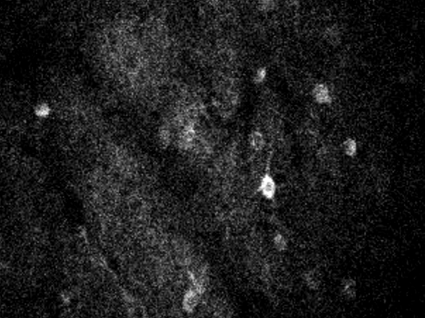
Ca imaging video, many cells
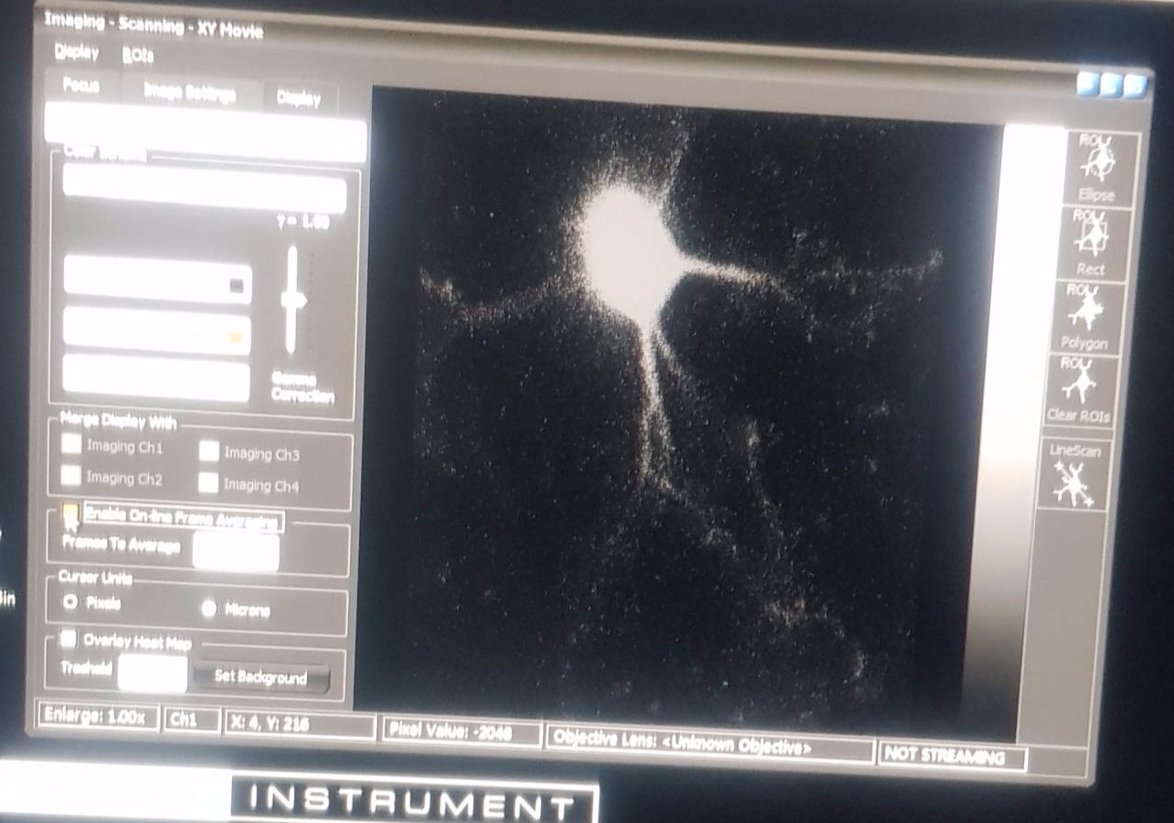
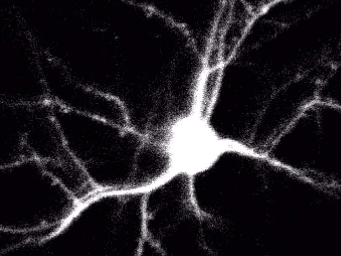
Ca imaging video, single cell
Ca imaging video, part of cell
Ca imaging video, many cells
Ca imaging video, single cell
A simple model of neuronal calcium dynamics
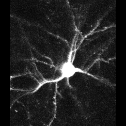
In the experiments we saw images of neurons flashing when responding to certain visual stimuli. The interpretation of these experiments is that: (1) a flash indicated elevations in the intracellular Ca2+ concentration ([Ca2+]) , (2) the [Ca2+] elevation indicated that the neuron fired an action potential, and (3) the action potential indicated that the neuron received a sufficiently strong external input to drive it above firing its threshold.
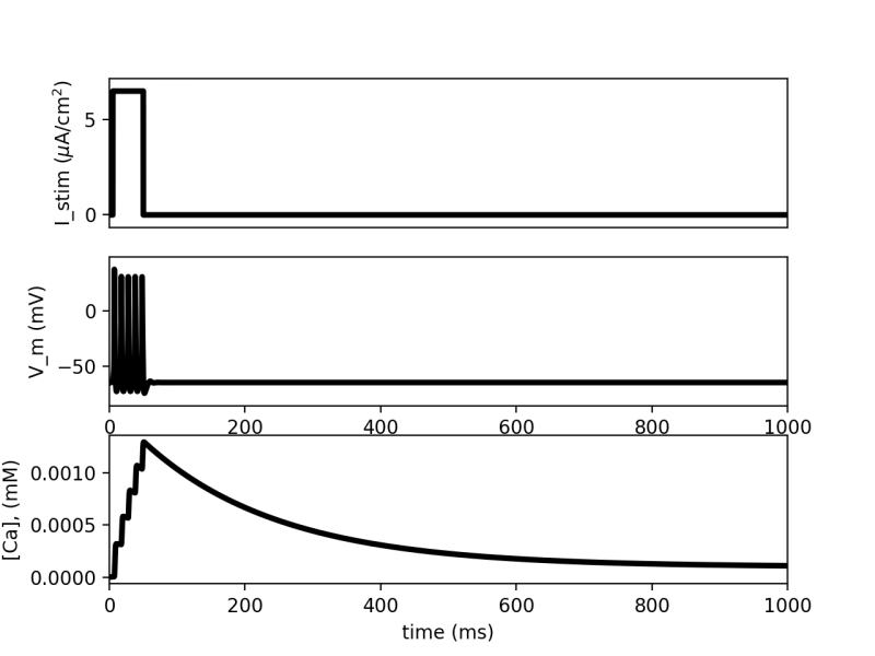
In this exercise, we will make a simple model that captures the relationship between the input, the action potential and the [Ca2+] dynamics in a neuron. We will use the good old Hodgkin-Huxley (HH) model for action potential generation as a starting point, and Your task is to expand this model to also include a Ca2+ channel and intracellular [Ca2+] dynamics.
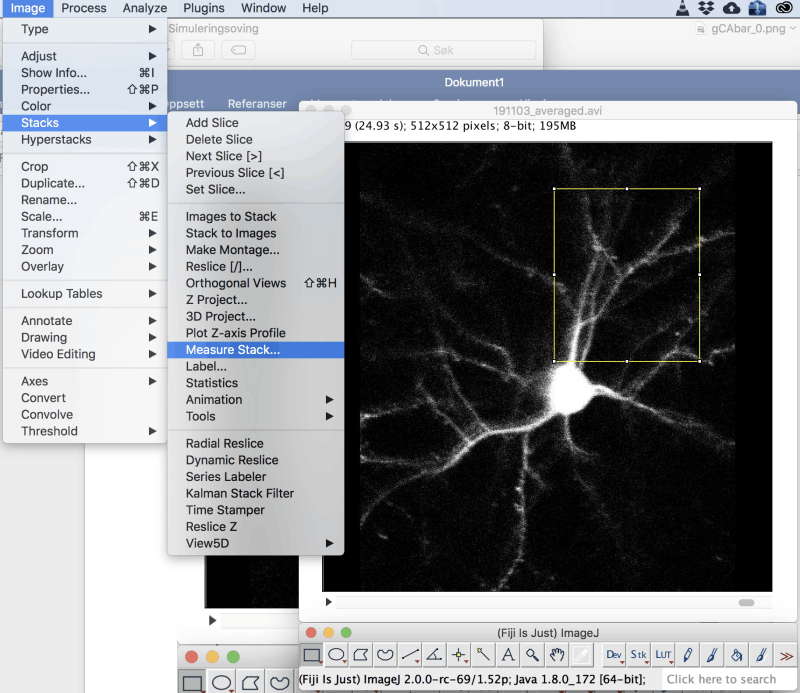

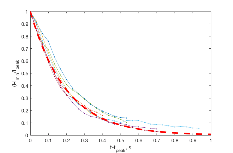
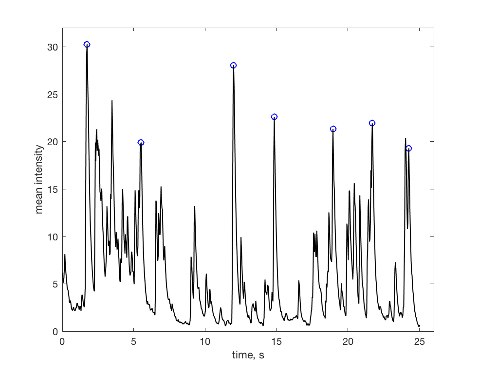
In the movie we picked out an area and measured the mean intensity in this area in all images. Plotting these intensities we got the intensity peaks above. The blue circles are the largest and best separated peaks. We then plot the normalized intensity for the decay of each of these peaks marked with blue circles.
One observes that they all have a similar decay rate. The thick, red dashed line is an exponential exp(-t/tau), tau=0.2. Using this decay rate in the simulations one observes that the simple exponential decay in the model (right hand figure) is now fitted to the experiments.